Rigid-body Transformations

In the previous section, we introduced the idea of two different coordinates systems we called voxel-space and world-space. In order to use both systems, we need to be able to convert between them. As such, we need to be able to take voxel coordinates and convert them into millimetres, as well as take millimetre coordinates and convert them into voxels.

Very generally, the ability to transform coordinates from one system into another can be expressed as

\[\begin{split} \begin{align} b_x &= m_{11}a_x + m_{12}a_y + m_{13}a_z + m_{14} \\ b_y &= m_{21}a_x + m_{22}a_y + m_{23}a_z + m_{24} \\ b_z &= m_{31}a_x + m_{32}a_y + m_{33}a_z + m_{34} \end{align} \end{split}\]

where \(a_x\), \(a_y\), \(a_z\) represent the original coordinates and \(b_x\), \(b_y\), \(b_z\) represent the transformed coordinates. You might recognise each new coordinate as a linear combination of the old coordinates and some values called \(m\). You might also recognise that this is therefore a system of three linear equations, which can be represented using matrices. As such, we can compactly represent this transformation in the form \(\mathbf{b} = \mathbf{Ma}\), which we can expand to

\[\begin{split} \begin{bmatrix} b_x \\ b_y \\ b_z \\ 1 \end{bmatrix} = \begin{bmatrix} m_{11} & m_{12} & m_{13} & m_{14} \\ m_{21} & m_{22} & m_{23} & m_{24} \\ m_{31} & m_{32} & m_{33} & m_{34} \\ 0 & 0 & 0 & 1 \end{bmatrix} \begin{bmatrix} a_x \\ a_y \\ a_z \\ 1 \end{bmatrix}. \end{split}\]

The matrix \(\mathbf{M}\) therefore contains the 12 parameters of the transformation (noticing that we have to add an extra row to make the matrix multiplication work). Multiplying a vector containing our original coordinates by \(\mathbf{M}\) will give us the coordinates transformed into the alternative space. We can also use \(\mathbf{M}^{-1}\) to convert from the transformed coordinates back into the original coordinates using \(\mathbf{a} = \mathbf{M}^{-1}\mathbf{b}\).

Affine Transformations

The parameters in the matrix \(\mathbf{M}\) encode what is known as an affine transformation. The word affine means that parallel lines remain parallel after transformation. As such, operations such as bending are not allowed. Transformation can therefore only be constructed by combining:

• Translations

• Rotations

• Zooming/Scaling

• Shearing

Examples of each of these operations are shown in Fig. 8.

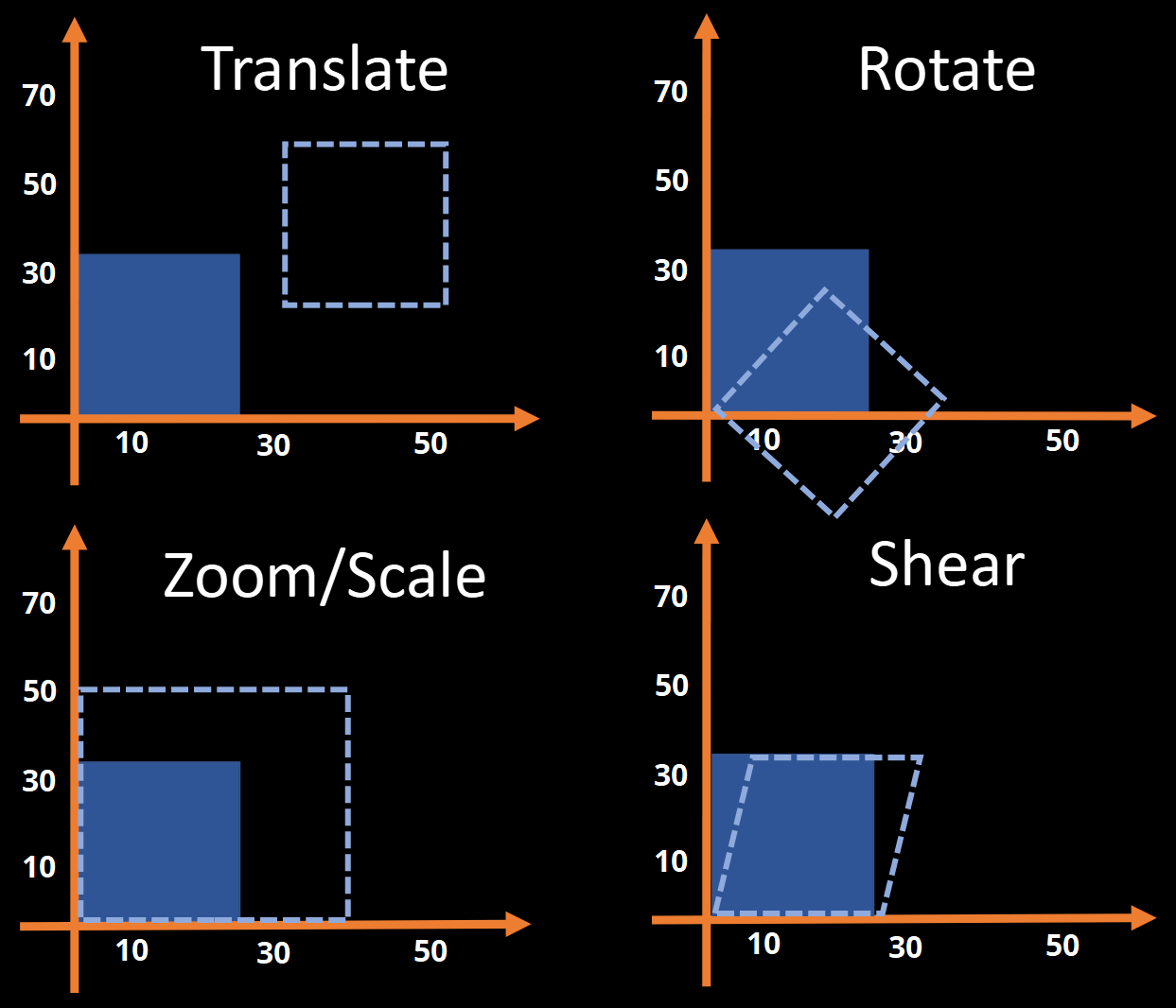
Fig. 8 Illustration of the operations that are allowed when forming an affine transformation.

To get a feel for affine transformations, you can play around with the example below. Move the sliders to change the transformation matrix, which is then used to change the coordinates of every pixel in the image.

Building an affine transformation within the matrix \(\mathbf{M}\) can be achieved by multiplying separate matrices that encode translations, rotations, zooms and shearing. As such, the final matrix has the form

\[ \mathbf{M} = \mathbf{M}_{T} \times \mathbf{M}_{R} \times \mathbf{M}_{Z} \times \mathbf{M}_{S}. \]

Each one of these individual matrices has a specific form, which can read about in the drop-down below.

Advanced: The Structure of the M Matrix

In terms of understanding how the \(\mathbf{M}\) matrix is formed, we can explore the structure of the individual matrices \(\mathbf{M}_{T}\), \(\mathbf{M}_{R}\), \(\mathbf{M}_{Z}\) and \(\mathbf{M}_{S}\).

To begin with, translating an image by \(q_{x}\) units along the \(x\)-axis, \(q_{y}\) units along the \(y\)-axis and \(q_{z}\) units along the \(z\)-axis would result in

\[\begin{split} \mathbf{M}_{T} = \begin{bmatrix} 1 & 0 & 0 & q_{x} \\ 0 & 1 & 0 & q_{y} \\ 0 & 0 & 1 & q_{z} \\ 0 & 0 & 0 & 1 \end{bmatrix}. \end{split}\]

Similarly, a rotation of \(q\) radians around either the \(x\)-axis (pitch), the \(y\)-axis (roll) or the \(z\)-axis (yaw) would result in

\[\begin{split} \mathbf{M}_{R_{x}} = \begin{bmatrix} 1 & 0 & 0 & 0 \\ 0 & \cos(q) & \sin(q) & 0 \\ 0 & -\sin(q) & \cos(q) & 0 \\ 0 & 0 & 0 & 1 \end{bmatrix},\quad \mathbf{M}_{R_{y}} = \begin{bmatrix} \cos(q) & 0 & \sin(q) & 0 \\ 0 & 1 & 0 & 0 \\ -\sin(q) & 0 & \cos(q) & 0 \\ 0 & 0 & 0 & 1 \end{bmatrix},\quad \mathbf{M}_{R_{z}} = \begin{bmatrix} \cos(q) & \sin(q) & 0 & 0 \\ -\sin(q) & \cos(q) & 0 & 0 \\ 0 & 0 & 1 & 0 \\ 0 & 0 & 0 & 1 \end{bmatrix}, \end{split}\]

with

\[ \mathbf{M}_{R} = \mathbf{M}_{R_{x}} \times \mathbf{M}_{R_{y}} \times \mathbf{M}_{R_{z}}. \]

You do not need to worry about all the trigonometry here. The main point is about the structure, in that rotations are encoded in both the diagonal and off-diagonal rows corresponding to the axes we are not rotating around.

Zooms by a factor of \(q_{x}\), \(q_y\) and \(q_z\) are encoded in the diagonal elements, where a negative zoom will flip the axis. This operation is also referred to as scaling and is encoded using

\[\begin{split} \mathbf{M}_{Z} = \begin{bmatrix} q_{x} & 0 & 0 & 0 \\ 0 & q_{y} & 0 & 0 \\ 0 & 0 & q_{z} & 0 \\ 0 & 0 & 0 & 1 \end{bmatrix}. \end{split}\]

Finally, shears are encoded using parameters in the top three off-diagonal elements

\[\begin{split} \mathbf{M}_{S} = \begin{bmatrix} 1 & q_{1} & q_{2} & 0 \\ 0 & 1 & q_{3} & 0 \\ 0 & 0 & 1 & 0 \\ 0 & 0 & 0 & 1 \end{bmatrix}. \end{split}\]

Note that we are often interested in transformations that move the brain, without changing its general size or shape. These forms of transformation are known as rigid-body and correspond to a subset of affine transformations that do not include shearing. Furthermore, zooms are only allowed to use the same value of \(q\) for each axis, such that the brain can be scaled up and down, but not stretched or squashed.

Converting Between Voxel-space and World-space

Now that we have seen how affine transformations work, we can get back to the idea of converting between voxel-space and world-space. The key thing to understand is that this conversion is just an affine transformation, consisting of translating, rotating and scaling the axes so they represent millimetres instead of voxels. This process is illustrated in Fig. 9.

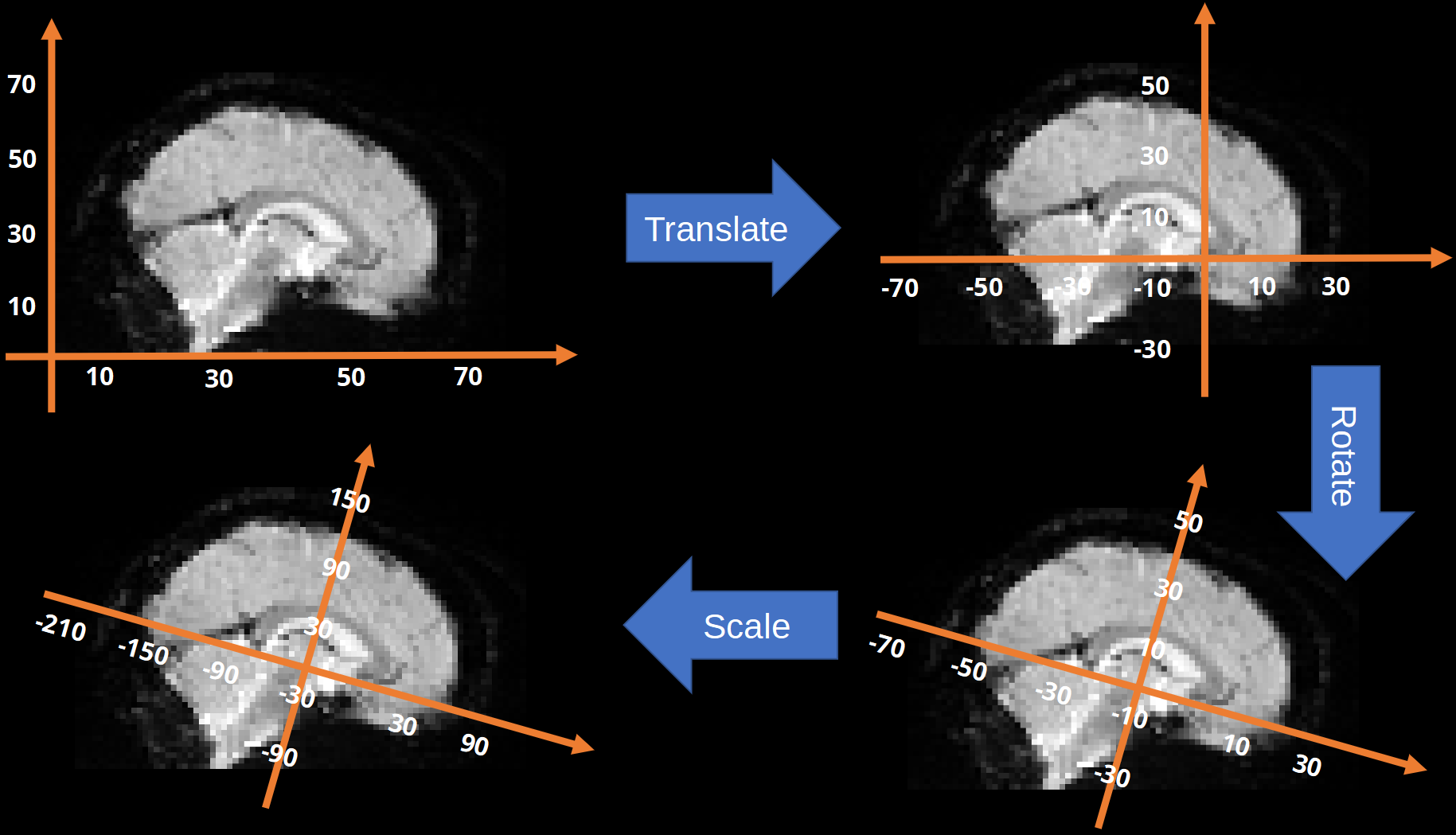
Fig. 9 Illustration of the affine transformation used to covert between voxel-space and world-space.

Given this, all we need to convert voxels into millimetres is a suitable \(\mathbf{M}\) matrix. We can then multiply voxel coordinates by \(\mathbf{M}\) and get the corresponding millimetre coordinates, as well as multiply millimetre coordinates by \(\mathbf{M}^{-1}\) and get the corresponding voxel coordinates.

So where do we get \(\mathbf{M}\) from? The answer is that most medical imaging file formats store all the necessary information from the scanner to create \(\mathbf{M}\). This information is stored in the metadata of the file, which is simply all the information carried within the file in addition to the voxel values. On this course, we will be mostly using the NIfTI format for brain images, which contains a voxel-to-world mapping matrix within its header information. Practically, this means that any NIfTI-formatted image carries with it the \(\mathbf{M}\) matrix needed to convert voxel coordinates into millimetre coordinates.

Tip

Remember that that data in voxel-space can be in any orientation because it depends upon how the data have been saved in the file. In all our examples we will assume, for simplicity, that the voxel-space data is correctly oriented. However, in cases where it is not, the affine matrix in the header will have some of the rows swapped. For example

\[\begin{split} \mathbf{M} = \begin{bmatrix} 0 & 3 & 0 & -20 \\ -3 & 0 & 0 & 110 \\ 0 & 0 & 3 & -190 \\ 0 & 0 & 0 & 1 \end{bmatrix}. \end{split}\]

This means that the voxel coordinates will be rearranged as part of the conversion to world-space. This means that the world-space coordinates will always be in the correct order, even if the voxel-space coordinates are not.

As an example, consider the MATLAB code below. First, we can extract \(\mathbf{M}\) from the header

hdr = spm_data_hdr_read('example_image.nii');
M   = hdr.mat

M = 4x4 double
    0.0122    0.0027    1.1999 -107.6227
   -0.7913    0.6113    0.0096   18.4938
    0.6113    0.7914   -0.0116 -191.0988
         0         0         0    1.0000

Then we use \(\mathbf{M}\) to convert the voxel coordinates \([20, 25, 30]\) to millimetre coordinates

coords.mm = M * [20 25 30 1]';
coords.mm

ans = 4x1 double
  -71.3129
   18.2397
 -159.4359
    1.0000

Finally, can use the inverse of \(\mathbf{M}\) to get from millimetres back to voxels

coords.vox = inv(M) * coords.mm;
coords.vox

ans = 4x1 double
   20.0000
   25.0000
   30.0000
    1.0000

Advanced: Breaking Down an M Matrix

SPM contains a function called spm_imatrix that takes an \(\mathbf{M}\) matrix as input and then returns the translation, rotation, scaling and shearing parameters for each axis. If you want to get a better understanding of how \(\mathbf{M}\) is formed, you can try running p = spm_imatrix(hdr.mat) to extract the parameters, and then building the \(\mathbf{M}\) matrix from the equations given earlier. For instance, you can form the matrix \(\mathbf{M}_{T}\) using

MT = [1 0 0 p(1); ...
      0 1 0 p(2); ...
      0 0 1 p(3); ...
      0 0 0 1]; 

and the matrix \(\mathbf{M}_{R_{x}}\) using

MRx = [1  0         0         0; ...
       0  cos(p(4)) sin(p(4)) 0; ...
       0 -sin(p(4)) cos(p(4)) 0; ...
       0  0         0         1];

Continue like this for the remaining matrices and then try calculating

MR = MRx * MRy * MRz;
M  = MT * MR * MZ * MS

and see if the result is the same as hdr.mat.