Interpolation#
In the previous sections, we looked at how to map coordinates between different spaces and saw how we could use this mapping to perform a transformation in voxel-space. However, during this step we glossed over quite an important detail. In the example, we showed how the voxel coordinates changed for a shift of 9mm. This was chosen very specifically to be an exact multiple of the voxel size. But what happens if we want to move the image by some other amount? What if we want to move the image by 8mm, or 3.75mm, or any other value that is not an exact multiple of the voxel size?
To see what happens, first we will define a \(\mathbf{T}\) to enact a translation of 8mm backwards along the \(y\)-axis
We will define \(\mathbf{Q}\) in the same fashion as the previous section, and then transform the same coordinates \(\mathbf{a}\) to give
Make sure you take a moment to consider why this result is problematic. Remembering that \(\mathbf{Q}\) transforms voxel coordinates from the new space into voxel coordinates from the old space, we have an issue because there is no voxel 22.667 in the original image. In fact, this cannot exist because voxel coordinates are indices into the data matrix and therefore cannot have fractional values. As such, if we wanted to use this \(\mathbf{Q}\) to created a voxel-space transformation, what can we do?
The answer is that we have to estimate what value would be 66.7% of the way between voxels 22 and 23 in the original image. This estimation procedure is known as interpolation (sometimes called resampling, regriding or reslicing). When we interpolate a value we have to use the voxel values surrounding the desired point to make an informed decision about what value voxel 22.667 would have. This may sound unintuitive, given that voxel 22.667 does not exist. However, remember that when we measure the MR signal we are taking discrete samples of a signal that varies continuously across the brain. So, in reality, there would have been some value 66.7% of the way between our samples, we just did not measure it. As such, interpolation is about trying to recover the shape of the original spatial signal so we can estimate what this value might have been.
Tip
Interpolation is something you will come across in everyday life and is not just specific to medical images. For example, watching standard definition content on a high definition television. Standard definition has a resolution of \(720 \times 480\) pixels, whereas high definition is \(1920 \times 1080\) pixels. In order to get standard defintion content to fill the screen, it needs to be zoomed by a factor of \(2.667\) along the \(x\)-axis and \(2.25\) along the \(y\)-axis. This will require some form of interpolation, which explains why such images will appear blurry when blown up because interpolation will not add any information to the image. This means that detail cannot be created to compensate for the larger image size. Furthermore, the zoom factor is not the same across each axis, so the content will appear stretched. Alternatively, a factor of \(2.25\) can be used for the horizontal axis, with any pixels that are out-of-bounds coloured black. This will result in vertical black bars at the side of the screen in order to maintain the original aspect ratio of the image.
Nearest-neighbour Interpolation#
The first and most basic approach we could take to finding a value for voxel \([20, 22.667, 20]\) is to pick the value closest to these coordinates. This is the same as rounding the coordinates, so when faced with coordinates \([20, 22.667, 20]\) we round them to the nearest whole-numbers to give \([20, 23, 20]\). The voxel at \([20, 23, 20]\) is therefore the nearest-neighbour to our desired point and thus becomes the value we use as our estimate.
The biggest advantage of nearest-neighbour interpolation is that it is very simple and computationally fast. Nearest-neighbour is also the only interpolation method that does not create new values, as the interpolated values are only ever repeats of what was originally in the image. All other interpolation methods can create new values that were never in the image in the first place. As such, for cases where you want to preserve the original data values, nearest-neighbour is the only choice.
Nearest-neighbour interpolation is visualised in Fig. 10. On the left is a graph showing interpolation in a single dimension, where the green circles represent the original voxel values and the dashed lines represented the in-between values estimated by nearest-neighbour interpolation. On the right is an example of an image that has been interpolated using the nearest-neighbour approach. Notice that is has a characteristically “blocky” appearance, which matches with the sharp changes in values shown in the graph. Remembering that the aim of interpolation is to try and recreate the original spatial signal, it is unlikely that the true signal looked like the dashed line. Nearest-neighbour is therefore the most inaccurate interpolation method, from both a signal-recreation perspective and a visual perspective.
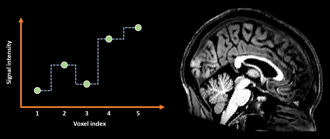
Fig. 10 Illustration of nearest-neighbour interpolation applied in 1D (left) and to an image (right).#
Linear Interpolation#
A more sophisticated method for finding a value for voxel \([20, 22.667, 20]\) is to consider how far this voxel is from its neighbours and use that information to determine a value. In this example, 22.667 is 66.7% of the way between 22 and 23. So, what we could do is plot a straight line between the value of voxel \([20, 22, 20]\) and voxel \([20, 23, 20]\) and then see what new value sits 66.7% of the way along this line. This is the essence of linear interpolation.
Advanced: The Maths of 1D Linear Interpolation
When working in one dimension, the interpolated value is given by
where \(c_c\) is the fractional coordinate, \(c_a\) is the coordinate below \(c_c\), \(c_b\) is the coordinate above \(c_c\), \(v_a\) is the voxel value at \(c_a\) and \(v_b\) is the voxel value at \(c_b\). To see this in action, consider our example of a coordinate of 22.667 and say that the value at voxel 22 was 5 and the value at voxel 23 was 7. The interpolated value would be
which makes sense because the difference between 5 and 7 is 2 and 66.7% of 2 is 1.334. So 66.7% of the way between 5 and 7 is \(5 + 1.334 = 6.334\).
When applied in 2D, this is often termed bilinear interpolation and involves performing several of the linear interpolations described above. For example, in the situation illustrated in Fig. 11 we have 4 points labeled A-D and an in-between point labeled G. To find a value for G, we first use linear interpolation between A and B to find the point E and then use linear interpolation between C and D to find the point F. We then interpolate between E and F to find our final value of G.
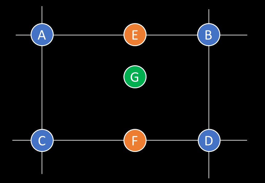
Fig. 11 Illustration of linear interpolation in 2D (often called bilinear interpolation).#
This process can be generalise to 3D (termed trilinear interpolation) by doing a bilinear interpolation in the slice above and below the fractional coordinates, and then doing a linear interpolation between the results of the bilinear interpolations.
Linear interpolation is visualised in Fig. 12. Notice how in the graph the dotted lines show a smoother transition from one value to another compared to nearest-neighbour interpolation. This smoothness is reflected in the much smoother appearance of the image on the right. This visual improvement of linear interpolation over nearest-neighbour is why this method is often favoured for visualising images. However, thinking back to the idea of recreating the original spatial signal, linear interpolation is still soemwhat inaccurate, as it is unlikely that the original spatial signal consisted of perfectly straight lines between the chosen sampled points. As such, linear interpolation is more accurate that nearest-neighbour from a visual perspective, but could still be improved from a signal-recreation perspective.
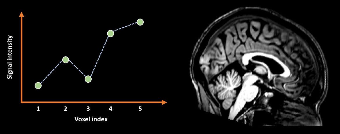
Fig. 12 Illustration of linear interpolation applied in 1D (left) and to an image (right).#
B-spline Interpolation#
To move beyond simple nearest-neighbour and trilinear interpolation, we can consider methods of generalised interpolation (Thévenaz, Blu & Unser, 2000). These are methods that include both of the classical interpolation techniques described above, but also allow for much higher quality interpolation as well. The generalised interpolation method favoured by SPM is known as B-spline interpolation. Without getting too deep into the details, the main point about B-splines is that they have a property called the degree, which is associated with the number of neighbouring voxels used to define the interpolated value. A B-spline of degree \(n\) uses \(n + 1\) neighbours to define its shape. This means that for degree 0, only 1 neighbour is used and is therefore the same as nearest-neighbour interpolation. For degree 1, only 2 neighbouring voxels are used and thus is equivalent to linear interpolation. As we increase the degree we produce a theoretically more accurate estimation of the original signal, as more data are used to estimate it. The only cost is that higher degree interpolation is slower to compute.
Higher-degree B-spline interpolation is visualised in Fig. 13. Notice how in the graph the dotted lines are similar to linear interpolation, but with smoother peaks and troughs around the actual data points. The visual improvement afforded by this extra smoothness is very subtle, however, the theoretical improvement in the estimated shape of the underlying signal is enough to justify this form of interpolation as preferable over both linear and nearest-neighbour methods. However, it is worth considering that the smoothness around the troughs of the signal can cause B-spline interpolation to dip below 0 and thus produce negative values, even if the values in an image are all positive. This will not happen with either linear or nearest-neighbour. As such, for data that only makes sense when it is positive, B-spline may not be the best choice.
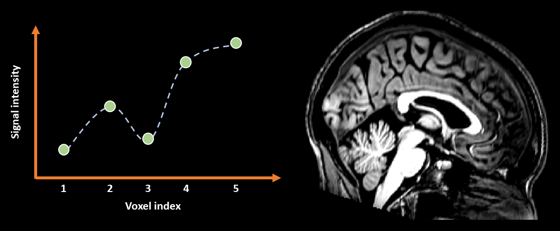
Fig. 13 Illustration of 3rd-degree B-spline interpolation applied in 1D (left) and to an image (right).#
Interpolation issues#
Interpolation, though necessary, is a procedure that we have to treat with caution. One of the bigger issues we can face is interpolating the same dataset too many times. Notice in the examples of interpolation above that the image gets blurrier after resampling. If we were to resample the image again and again this blurring would get progressively worse. This indicates a loss of information after each interpolation step. In effect, we are degrading the data. This is particularly problematic when working with images from modalities such as PET or fMRI, where the resolution is already low. As such, we have to take care to only resample our data as many times as absolutely necessary.
An illustration of this issue can be seen in Fig. 14. Here we can see how successive interpolation results in a loss of data and blurring of the image. The alternative is therefore to concatenate multiple transformations and then only resample the data once. In Fig. 14, concatenation reveals that that no changes are need and so no image degredation is necessary.
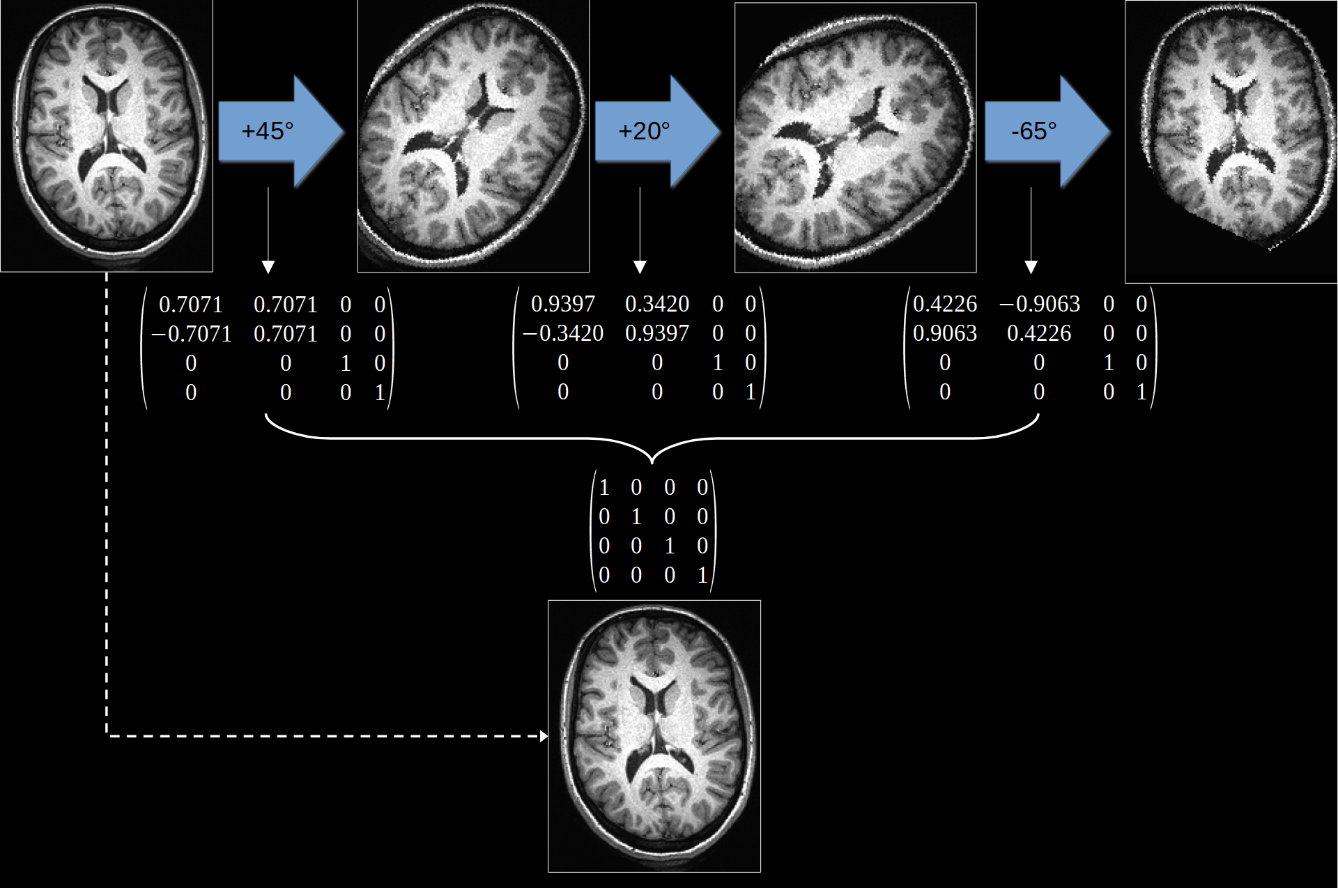
Fig. 14 Illustration of how applying multiple transformations can degrade a dataset. Instead, we can concatenate mutiple transformations together before applying them. In this example, the transformations cancel and thus no interpolation was actually necessary.#