Image Filtering#
We are now going to move on from spatial transformations to talk about image filtering. We are not going to spend as mutch time on filtering because spatial transformations are both more common and are also the source of more errors compare to filtering. That being said, filtering is still frequently used and discussing it here will allow us to first approach topics such as convolution, which will come in handy later in the course.
We will be mainly discussing filters in their most intuitive form within the spatial domain. This means we are dealing with methods that directly change the voxel values of the image. We will introduce the idea of filters within the frequency domain a little later on, for those who would like a slightly different perspective. However, the main point is to understand how filters can be applied spatially to an image.
Kernels#
The key to understanding how image filtering works is to understand the concept of a kernel. A kernel is a small matrix used to weight the voxel values to produce new values in an image. The idea is that we slide the kernel across the image and then calculate a new value for the voxel the kernel is centred on, using all the voxels the kernel is covering.
As an example, we are going to use a Gaussian kernel, which is used in neuroimaging to smooth or blur images. Smoothing is a technique to reduce noise in an image because the Gaussian kernel performs a weighted averaging of neighbouring voxels. This means that random noise across voxels will tend to cancel-out, whereas values that are consistent across voxels will tend to remain. An example of a 3 x 3 Gaussian kernel is shown below
The values in the kernel are derived from a Gaussian distribution (also known as the normal distribution), which is easier to see when visualised in 3D, as shown in Fig. 15 for a \(17 \times 17\) kernel.
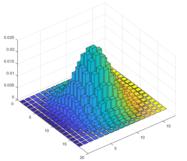
Fig. 15 Illustration of a \(17 \times 17\) Gaussian kernel.#
Note that the width of a normal distribution is usually controlled by its standard deviation (represented by \(\sigma\)). In neuroimaging, however, it is more typical to talk about the Full Width at Half Maximum (FWHM) value in the context of a smoothing kernel. This value gives the number of voxels the kernel covers at half its height, as illustrated in Fig. 16. Parameterising the kernel in this fashion means we can think about the coverage of the kernel more intuitively in terms of voxels. The standard deviation and FWHM are connected, as shown by the formula
You do not need to memorise this, but it is just useful to know that the two concepts are connected.
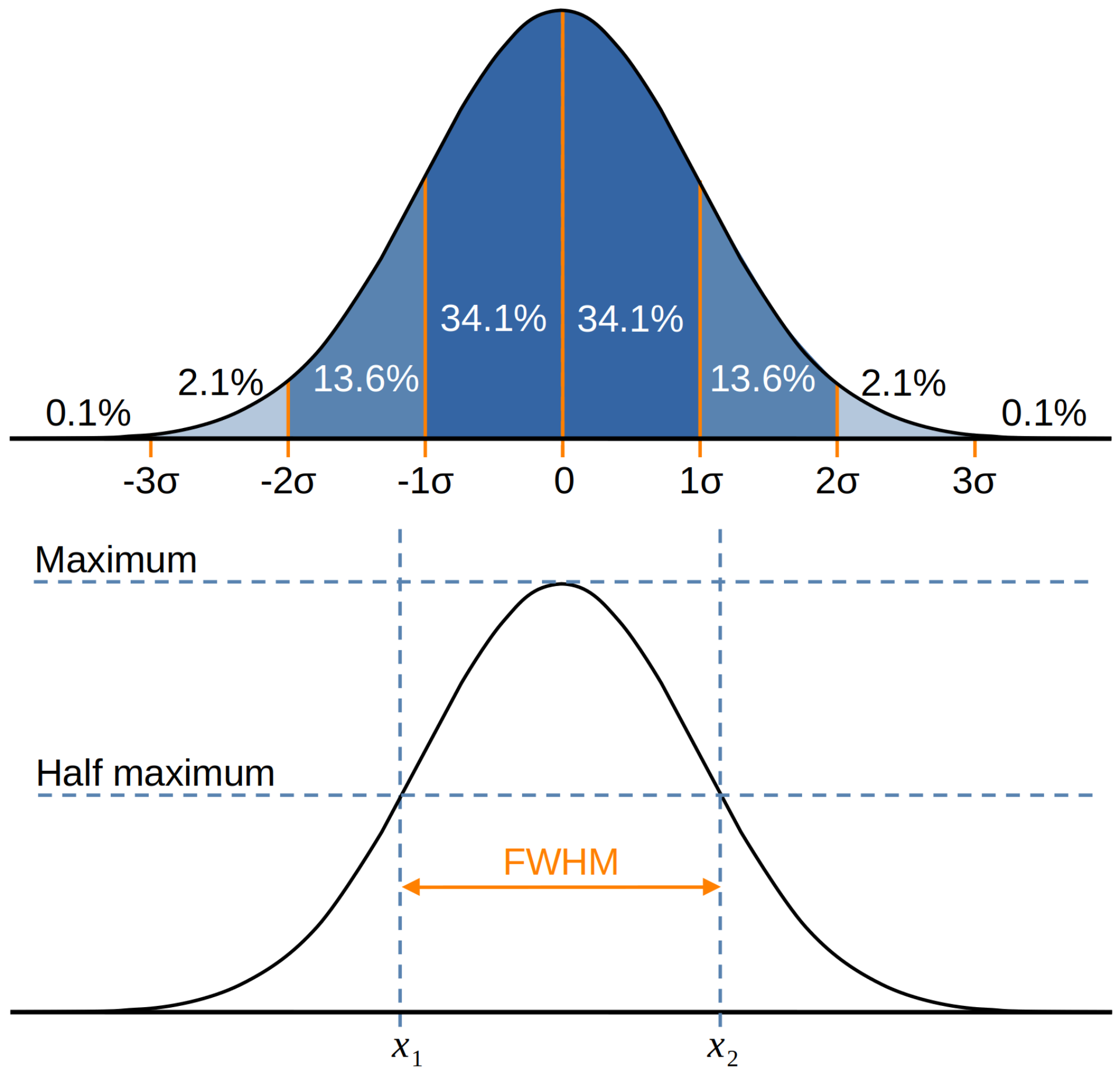
Fig. 16 Illustration of how the FWHM is defined in terms of a Gaussian distribution and how it relates to the standard deviation.#
In terms of how this kernel would be used to smooth an image, Fig. 17 tries to visualise the process. We can see that the kernel is placed over a patch of voxels and then the overlapping values are multiplied and summed to produce a value of 123.77. This process is more formally known as convolution and will be explored a little more below. The number 123.77 becomes the new value of the voxel the kernel is centred on, as indicated by the arrow. Continuing through the image in this manner produces the smoothed version of the image you can see on the right.
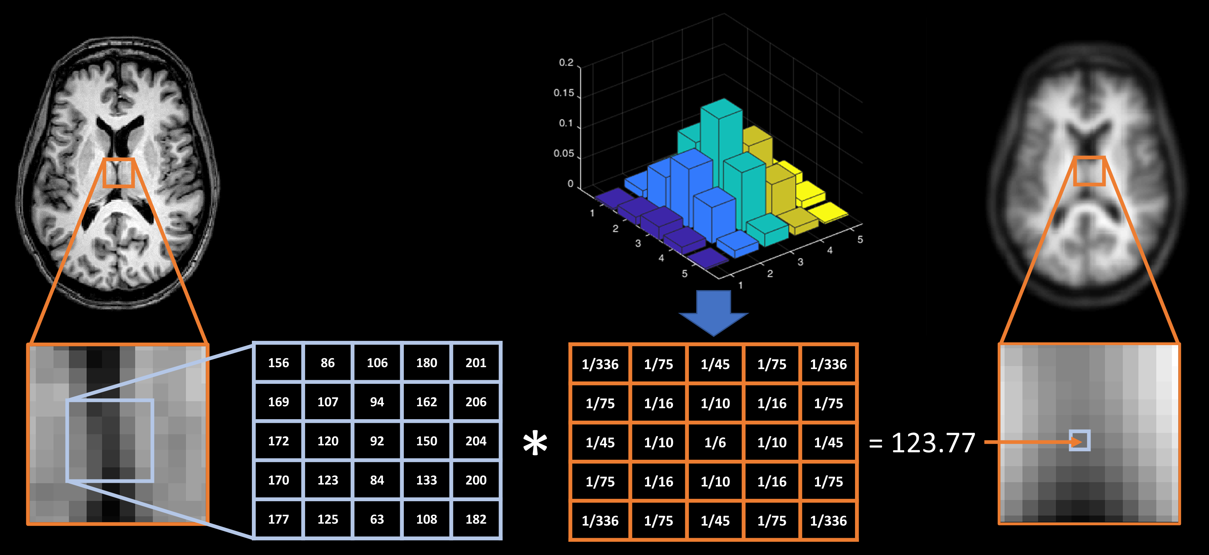
Fig. 17 Illustration of how smoothing is achieved via the process of convolving a Gaussian kernel with an image.#
Convolution#
As mentioned above, the process of multiplying a kernel and an image to produce a new value is an example of a more general mathematical procedure called convolution. This is a procedure that we are going to encounter in a few places on this course, so it is worth a little bit of time discussing it now. To formalise this, the 1D convolution of a Gaussian kernel (\(g\)) and an image (\(i\)) at voxel \(n\) would be written as
where the indices of the kernel run from \(-M\) to \(M\). All this means is that you should work through all the voxels that overlap between the kernel and the image, calculate the product of the overlapping values and then add them together.
The main thing to understand in the formula above is that \(i\) and \(g\) could be any functions. Convolution is a very general process that creates a new function from two input functions. In our example, the new function is the smoothed spatial signal and the inputs are the un-smoothed spatial signal and the kernel. However, these could be anything. For example, the GIF below shows the convolution of a square function and curved-triangle function.

The main thing to remeber is that the height of the result at each point is proportional to the area of overlap. So in this illustration, the height at each point is proportional to the yellow shaded area. As another example, the GIF below shows the convolution of two square functions, which produces a triangle thanks to the increasing and then decreasing overlap between the squares.

Hopefully the similarities to running a kernel over an image are clear in these examples. We will see convolution coming up again when we come to analysing fMRI data, so make sure you have some sense of how it works here as it will make the more complex fMRI application easier to understand.
Smoothing in SPM#
We have used smoothing as our filtering example in this section because this is one of the key steps that we will use when processing fMRI images. Although there are many other potential filters, the Gaussian filter has become a mainstay of neuroimaging data analysis. In SPM this is implemented as a convolution operation. In the video below you will see how to use the SPM smoothing module to apply a Gaussian filter to an image. Click here to download the dataset for this example.
Filters in the Frequency Domain#
Beyond conceptualising filters as spatial convolution, it is also possible to view filters within the frequency-domain. Here, we think about how filters affect both high-frequency and low-frequency spatial information. The outcome is the same as spatial filters and so this alternative perspective is mainly useful for understanding what filters are doing. As such, we have left this as an advanced topic for those who wish to know a bit more. You can read about this using the advanced drop-down section below.
Advanced: Filters in the Frequency Domain
Fourier analysis
The starting point for understanding frequency-domain filters is with Fourier analysis. Unfortunately, Fourier analysis is a difficult topic to fully appreciate without a fair amount of mathematical kowledge. However, at its core is a very simple principle. Imagine we had a cake and we wanted some way to unmix it to tell us what ingredients went into the cake, and how much of each ingredient went into the cake. Although we cannot do this with a real cake, Fourier analysis allows us perform this type of unmixing using any signal we want. The ingredients that go into the signal are periodic functions, such as sines and cosines. Using a Fourier transform of a signal, we can construct a power spectrum that tells us both the frequencies of these periodic functions, as well as their strength. Essentially, this tells us both the ingredients and the amount of each ingredient that make up any signal. Further more, the inverse Fourier transform allows us to go from those ingredients back to the original signal. What this mean is that we can break a signal down into its ingredients, remove any ingredients we do not want, and then build the signal back again with those bits removed.
To see this in action, let us start with a simple example. In Fig. 18 we have a cosine wave that cycles every 0.02 seconds (so 50 cycles per-second) on the top, and we have the Fourier transform of that wave on the bottom. As we can see, the power spectrum of this wave has a spike at 50Hz, which tells us that this signal is entirely constructed from a single periodic function with a frequency of 50Hz.
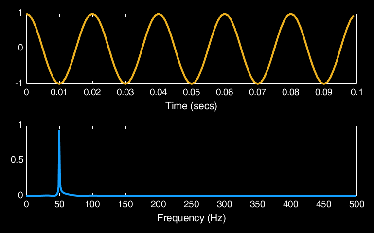
Fig. 18 Illustration of the Fourier transform of a signal composed of a single 50Hz cosine wave.#
In Fig. 19 we have a more complex example of a signal composed of a cosine wave with a frequency of 50Hz and another cosine wave with a frequency of 150Hz. These waves have been weighted by 0.7 and 0.3 respectively so that there is more of the 50Hz wave in the signal than the 150Hz wave. Looking at the Fourier transform, we can see that not only has it managed to unmix both of these signals, but has also given us the correct amount of those signals. What is useful about this is that If we were to remove the 150Hz spike from the power spectrum and then use the inverse Fourier transform, we would completely remove the 150Hz wave from the original signal.
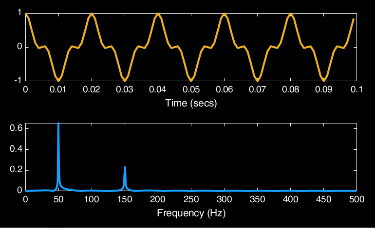
Fig. 19 Illustration of the Fourier transform of a signal composed of a 50Hz cosine wave and a 150Hz cosine wave.#
Frequency domain filtering
So now let us see how we can use a Fourier transform to filter images in the frequency domain. In Fig. 20 we have taken a row from a single slice of a structural MR image and have plotted the voxel values. This is the spatial signal that we will be smoothing. If we put this through the Fourier transform we get the power spectrum shown on the right. We can then take a Gaussian distribution, as used previously to derive the Gaussian kernel, and also put that through a Fourier transform to get its power spectrum.
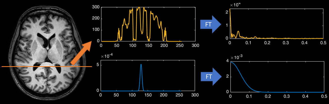
Fig. 20 Illustration of the Fourier transform applied to the 1D spatial signal taken from an MR image.#
The idea in the frequency domain is that we multiply the power spectrum of the signal and the power spectrum of the kernel. Hopefully you can see from the illustration in Fig. 20 that doing this will give preference to the low-frequencies and will completely remove any high-freqeuncies over a certain value. So let us see what happens when we perform thus multiplication and then convert the result back into the spatial domain. The result is given in Fig. 21

Fig. 21 Illustration of multiplying the power spectrums of the spatial signal and kernel, and then converting the result back to the spatial domain using the inverse Fourier transform.#
As we can see, we get a smoothed version of the spatial signal. This is identical to the results you would get if you convolved this signal with a Gaussian kernel. We can see that much of the detail has disappeared, as this corresponds to the high-frequency information in the signal. So all we are left with is low-frequency information, corresponding to the gross changes in signal intensity across the image. This means that the fine detail in the image will be gone, hence the image gets blurrier. Because this filter does not change the low-frequency components it is known as a low-pass filter (because it passes the low-frequency information). If the filter were flipped around so it passed over the high-frequency components, it would be known as a high-pass filter. So slightly confusingly, a low-pass filter removes high-frequency information and a high-pass filter removes low-frequency information.