The Structure of fMRI Data

Before we get started, it is useful to review the structure of fMRI data. In this lesson, we are going to be focussing on the spatial and temporal elements of fMRI datasets. As such, it is important that you have a solid understanding of these features before we go any further.

4D Images

At its most basic, an fMRI dataset is a collection of 3D volumes measured in rapid succession. The speed at which these volumes are collected is given by the TR of the scanning sequence. A typical BOLD sequence will have a TR of 2-3 seconds. This defines the sampling rate or temporal resolution of the data. Together, these 3D volumes form a 4D dataset, consisting of three spatial dimensions and a fourth time dimension. Each point in the dataset can therefore be indexed both by its spatial location, as well as when it was collected during the fMRI sequence. Each of the individual 3D volumes are therefore snapshots in time. A typical fMRI series may contain around 200 of these snapshots. For each voxel, there would therefore be 200 associated values, quantifying how the BOLD signal changed during the experiment at that point in the brain. This sequence of values is known as the fMRI time series (see Fig. 1) and is the raw data of most interest for the purpose of statistical analysis.

Note

Given the description above, it is worth taking a moment to consider the scale of the data we are working with. Consider an fMRI volume with dimensions \(60 \times 60 \times 40\). Now consider that each voxel in this volume is associated with 200 time series values. This gives \(60 \times 60 \times 40 \times 200 = 28,800,000\) data points in a single fMRI dataset. Now consider that there may be 20 subjects in the study, each with over 28 million data points each. This means a total of \(28,800,000 \times 20 = 576,000,000\) individual measurements to process and analyse.

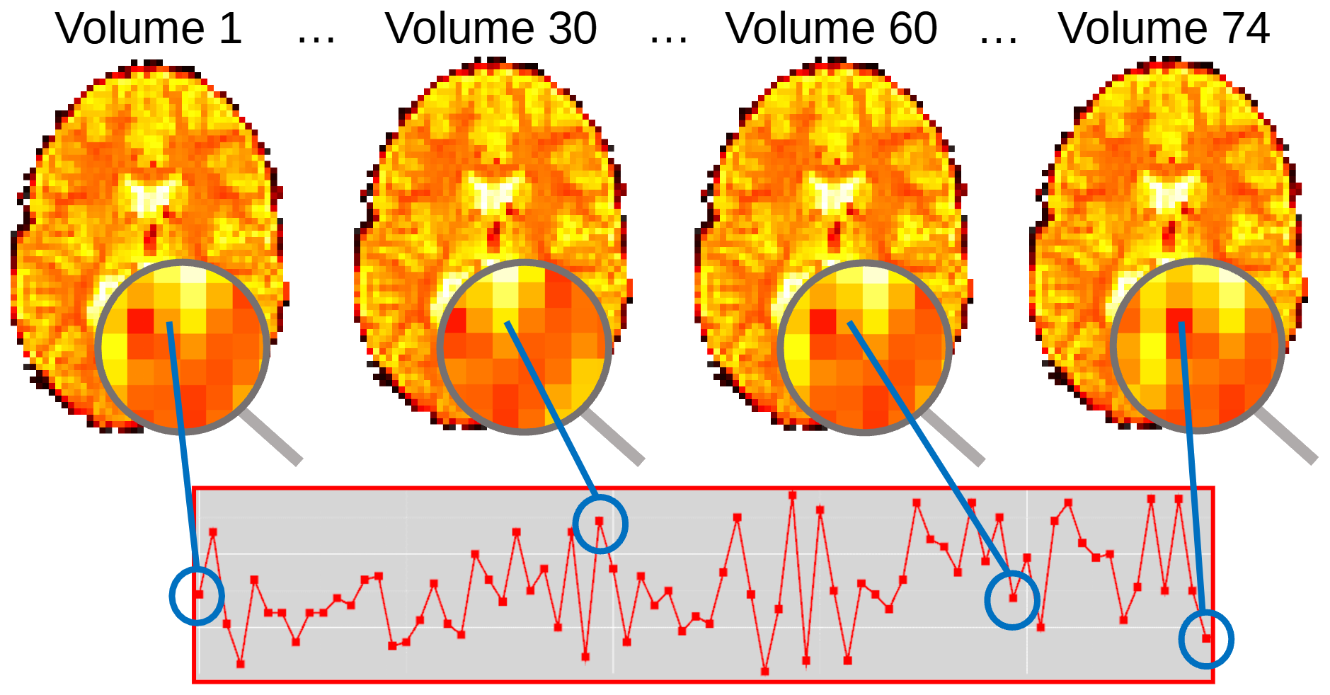
Fig. 1 Illustration of how each voxel in a functional image is associated with a timeseries of BOLD signal change.

Exploring an Example Dataset

To get a more solid understanding of how fMRI data are structured, download the functional and anatomical files that will be used as examples in this lesson. The video below will demonstrate how to explore this dataset using the SPM display facilities. Here you will see how to display an fMRI series as a movie of 3D volumes, as well as how to visualise the time series at each voxel.

The Need for Preprocessing

As well as understanding the structure of fMRI data, examination of raw images can also provide insight into why preprocessing is necessary. First of all, consider the GIF in Fig. 2. This shows a series of fMRI volumes as an animation. Notice the characteristic flickering. This flickering represents changes in signal intensity over time. In other words, it represents signal variance. The fact that the time series at each voxel changes over time is hardly surpising, however, this notion of change is central to understanding the information that the signal contains.

Fig. 2 Illustration of the variance at each voxel over time.

Fundamentally, the purpose of analysisng fMRI data is to understand why the value of the signal changes. In an ideal world, all signal change would be a result of the experimental manipulation. Unfortunately, the reality is that there are many other reasons why the signal may be changing over time. These could relate to noise from the scanner, motion from the subject or other aspects of physiology not connected to blood flow. Whatever the reasons, we conceptualise the variance of a time series \(\left(\sigma^{2}_{y}\right)\) as a combination of variance associated with the experiment \(\left(\sigma^{2}_{\theta}\right)\) and variance associated with other sources \(\left(\sigma^{2}_{\epsilon}\right)\). Formally, we would write

\[ \sigma^{2}_{y} = \sigma^{2}_{\theta} + \sigma^{2}_{\epsilon} \]

When it comes to our analysis, not only do we want to cleanly separate these sources, but we also want to minimise \(\sigma^{2}_{\epsilon}\). This is because this quantity represents our degree of uncertainty about the experimental effects. In most statistical analyses, it is the ratio of these sources that is most important. This is why, in part, we need preprocessing, to help minimise known sources of signal variance that are not associated with the experimental manipulation.

Beyond minimising sources of additional variance, preprocessing also aims to address a fundamental difficulty with multi-subject fMRI studies. Although the gross anatomy of the brain will be the same from subject-to-subject, the size and shape will not. This anatomical variability can be substantial, as shown in Fig. 3. This causes significant issues with the analysis and localisation of results across groups of scans. As such, it is typical to spatially normalise fMRI data so that the images from all subjects are in the same coordinate space. Becuase of this, the second aim of preprocessing is to move all subjects into the same space to meet the assumptions of later statistical analyses.

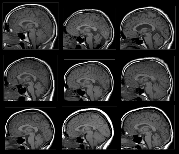
Fig. 3 Illustration of the variability in anatomy across different individuals.

Preprocessing Preliminaries

Before we begin exploring the standard preprocessing steps, there are a number of preliminary steps. Firstly, it is always better to work on copies of data, rather than the original files. Not only does this make it easier to start again if there are problems, but SPM can also make invisible changes to the image headers during processing that we will want to remove before starting again. Working with new copies each time is the easiest way to do this. SPM also creates a lot of new files during preprocessing and so it is useful to create a new folder to keep things organised. As such, the first preliminary step is to make a new folder and then create copies of the images inside that folder.

The next preliminary step is to examine the default registration between the functional and anatomical images. Many of the preprocessing steps we will discuss are forms of image registration and, as discussed earlier on the course, we can help the registration algorithms by first doing some rough manual alignment. This usually takes the form of setting the origins of both the functional and anatomical scans to the anterior commissure and then make any further orientation adjustments to bring the images into closer alignment in world-space.

Both of these preliminary steps are demonstrated in the video below.