Building the Preprocessing Pipeline

So far in this lesson, a rigid structure for preprocessing has been presented. Although this sequence of steps is applicable to most datasets, preprocessing should not always be blindly applied in this order. In this final section, we are going to present some key questions that should be asked whenever you are building a preprocessing pipeline. Depending upon the answers to these questions, the order of certain preprocessing steps may be reversed, or some steps may be skipped entirely. As such, it is important to recognise that preprocessing is not necessarily a fixed set of steps and that decisions need to be made to suit different datasets.

Do We Always Need Slice Timing Correction?

Earlier in this lesson we discussed the controversies surrounding slice timing correction, raising questions about whether this step should be used at all? This is a difficult question to answer as some authors, such as Poldrack, Mumford and Nichols (2011), recommend never using slice timing correction. Their argument is that with shorter TRs the slice timing problem is not as problematic as it once was, to the extent that we can accommodate the slice offsets within the statistical model without needing to correct the raw data. This also avoids issues with ringing artefacts and the other interpolation issues discussed earlier. Taken at face value, this argument seems to suggest that slice timing correction is a product of older scanning sequences that is no longer necessary for modern fMRI data analysis. However, we need to consider what evidence there is to support this position. In an effort to provide answers, a recent review was published by Parker & Razlighi (2019). This is an excellent paper and well worth reading in detail to understand the complexities of the slice timing problem. In summary, the authors found overwhelmingly that slice timing correction was beneficial, even in data collected with a short TR. The only situation where this is not the case is when data is collected using a block design experiment. We will discuss the exact nature of this type of experiment in the Experimental Design and Optimisation unit. The main point, for now, is that evidence has consistently shown very limited benefit to performing slice timing correction on block design data (e.g. Sladky et al., 2011). As such, if you are analysing data from a block design, slice timing correction can be skipped entirely. For all other types of data, the evidence suggests that slice-timing is always beneficial.

Should We Perform Slice Timing Correction or Motion Correction First?

Assuming that slice timing correction is appropriate for a particular dataset, questions arise about whether to perform slice timing correction first or motion correction first? If we return to the review by Parker & Razlighi (2019), their investigations suggested that it was often beneficial to perform motion correction first. The argument is that if we were to slice timing correct a timeseries that contains values from multiple regions of the brain, then the interpolation will effectively blur-together different regions of the brain across time. However, if there are large movements and the data were collected using an interleaved acquisition sequence, then things get more complicated. In this situation, the head motion will move different parts of the brain in and out of neighbouring slices. Because, in an interleaved sequence, these slices are sampled further apart in time, moving voxel across neighbouring slices during motion correction will mix together values measured at different time offsets. So we could end up with some values measured at the start of the TR and some measured near the end of the TR within the same timeseries. In this situation, slice timing correction will not be able to work correctly, meaning it may be better to perform slice timing correction first. As such, it is usually beneficial to perform motion correction first. However, if data were collected with an interleaved sequence and there are issues with large head motions, it may be better to perform slice timing correction first instead.

Note

In any situation where there are uncertainties about the preprocessing choices, a sensitivity analysis could be undertaken where the data are processed both ways and any consistencies or inconsistencies in the results are examined. This should reveal which findings are robust and which appear sensitive to the order of the preprocessing steps.

Should We Resample After Motion Correction?

During the motion correction section of this lesson, we discussed how the data can be resampled once all the \(\mathbf{T}\) matrices have been estimated. This effectively applies the motion correction to the data. In the context of this lesson, this was so that the slice timing correction was applied accurately after the motion correction. However, as indicated above, slice timing may come first in some pipelines, or may not be used at all. In these situations, it would be better not to resample the functional data. This is because we want to minimise the number of interpolation steps to prevent image degradation. Recall that an affine transformation is the first step in spatial normalisation. This initial affine transformation can be concatenated with the motion-correction transformations to produce a single initial affine step. This affine step can then be concatenated with the non-linear transformation to produce a single shift in the voxel-coordinates that only requires the data to be interpolated once. This effectively creates motion-corrected and spatially normalised images in a single interpolation step.

From a practical perspective, whenever you are performing slice timing first, or not at all, you can change the reslicing option in the Realign: Estimate & Reslice module to Mean Image Only, as shown in Fig. 24.

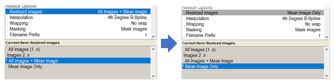
Fig. 24 Example of changing the reslice options for realignment.

SPM will then save or update the *.mat file containing the header matrices for each of the functional volumes. SPM will then automatically combined these transformation with those estimated by the Normalise module and the data will only be resampled once. From a practical perspective, this means that within the Normalise module you would select to apply the non-linear warping to the original functional files, rather than the ar*.nii or r*.nii files. In this situation, the final files from preprocessing would be named sw*.nii rather than swar*.nii or swr*.nii. Although it may seem like the motion correction has not been applied, this correction has in fact been combined with the normalisation step. As such, the w tag from the Normalise module indicates both motion correction and non-linear warping within the same step.

Preprocessing Flowchart

The flowchart in Fig. 25 provides guidance for preprocessing any data set with SPM. Although some of the issues and choices raised in this section apply, this pipeline should give you good quality results for the vast majority of datasets.

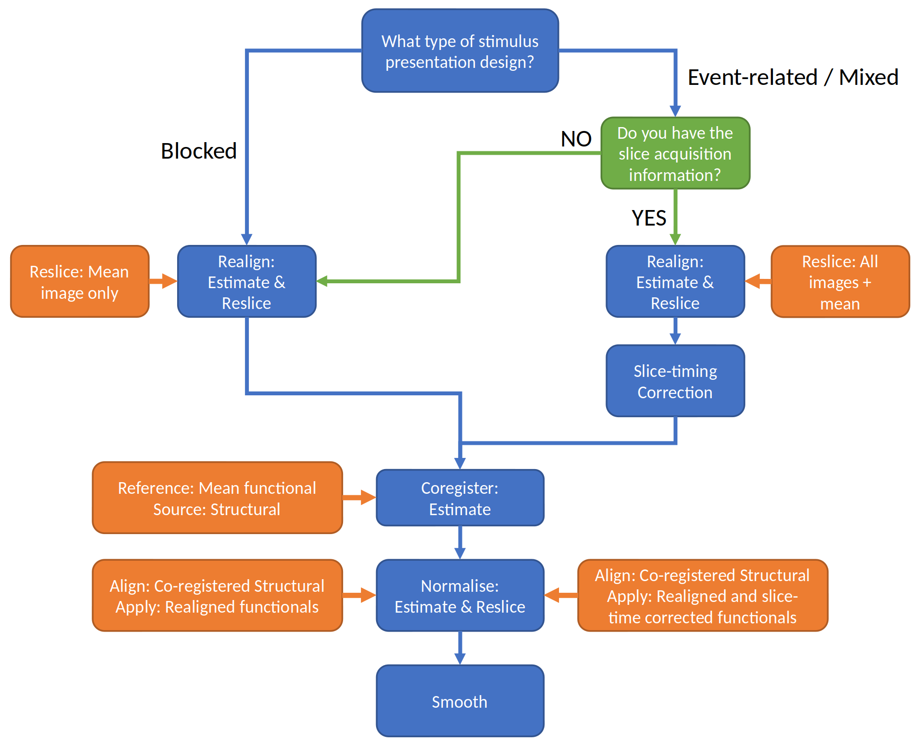
Fig. 25 A flowchart for performing preprocessing using SPM12.