Step 1: Motion Correction

One of the biggest sources of variance in the fMRI timeseries is head motion. Unfortunately, motion in the scanner is inevitable as it is unrealistic to expect all subjects to remain perfectly still for the duration of the experimental task. In cases where motion is particularly bad, it can cause such issues that the data cannot be used. Even in cases where the motion seems slight, changes in head position of as little as 2-3mm can corrupt the data. Motion is therefore a serious issue for the quality of our fMRI data. Although best to minimise movement at source, we must recognise that there will always be some head motion and must therefore be aware of what we can do to try and fix it.

Problems With Motion

There are two main issues resulting from head motion. The first is that motion will cause individual voxels to suddenly contain data from a different part of the brain. The second is that motion can disrupt the recording of the signal by the scanner. Both these issues can be further compounded by motion that occurs more during certain conditions of the experimental task. In these case, the motion is correlated with the task, creating a serious confound in the data.

Corruption of the Time Series

One of the main issue with motion is that the time series at an individual voxel is no longer a continuous measure of a specific point in the brain. Instead, the time series measures several points in the brain over time. Where this is particularly problematic is at tissue boundaries. For instance, motion may causes a voxel to contain signal from both inside and outside the head, or from both inside and outside the ventricles. In these cases, the change in tissue type will cause a sudden shift in signal intensity that may be misconstrued as true brain activity. This is shown in Fig. 4, where 20 volumes in the middle of a functional series have been artificially shifted to the right and then back again. Without any form of correction, the sudden change of intensity in the highlighted voxel would likely be identified as true brain activation by the statistical analysis.

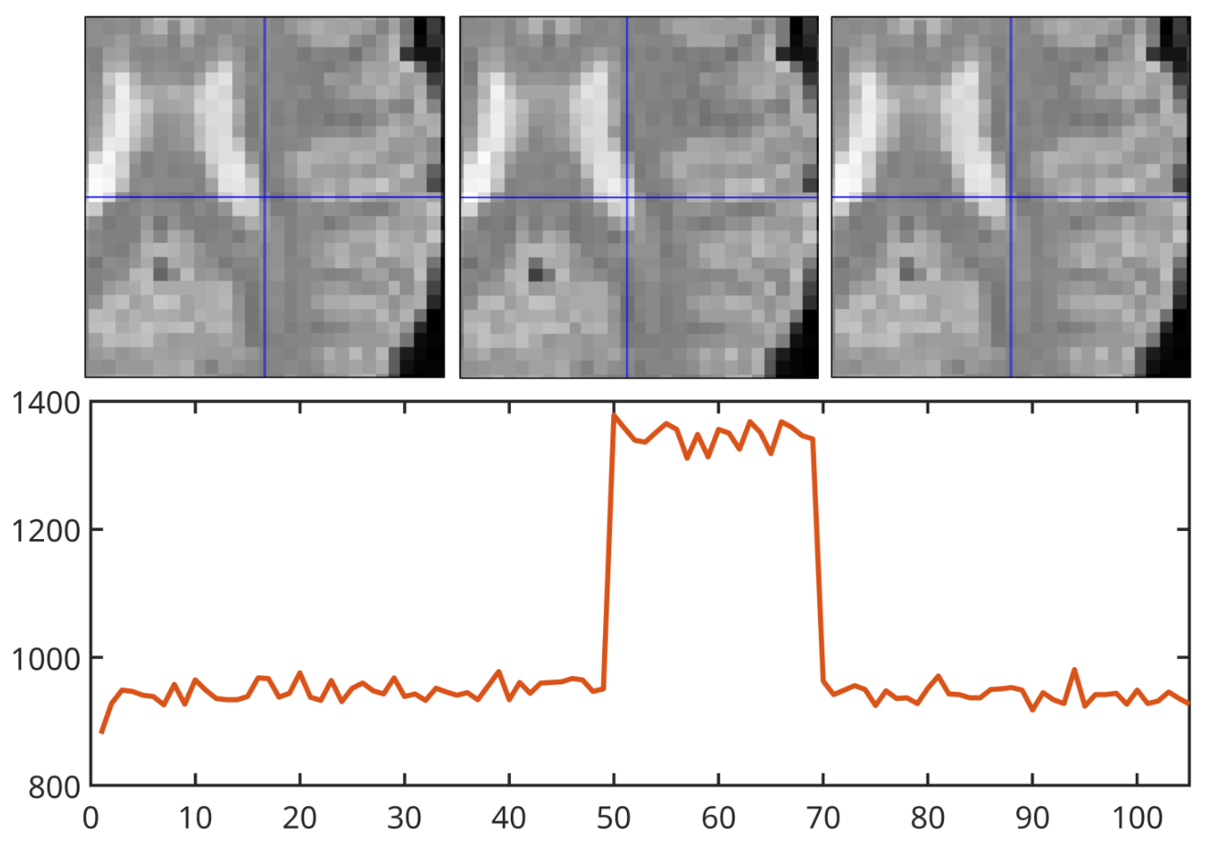
Fig. 4 Illustration of how sudden changes in signal intensity can occur after head motion.

One saving grace of this form of motion is that it is often visible as activations that trace the border between tissue types. As such, any activation pattern that sits along the edge of the brain, or along the edge of internal structures, should be treated with extreme caution. An example is shown in Fig. 5.

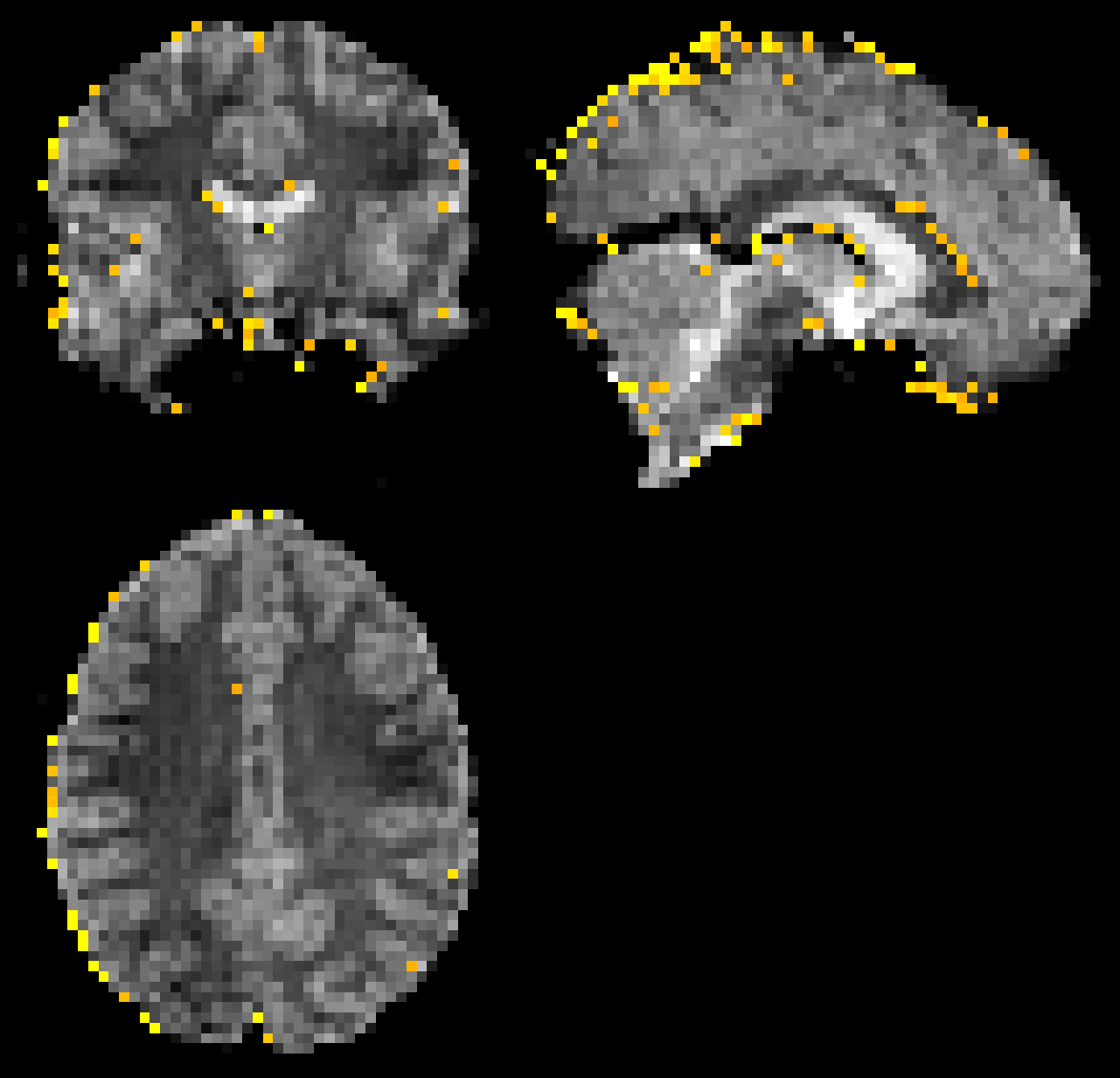
Fig. 5 Illustration of how motion artefacts can appear along the edges of the brain.

Corruption of the Signal Measurement

A more insidious effect of motion is that it can impact the signal measured by the scanner. When the subject’s head moves, protons from a neighbouring slice with a different excitation move into the voxel. This disrupts the magnetic gradients and alters the measured signal. This is exacerbated when using an inter-leaved acquisition sequence, as the excitation differences between neighbouring slices will be greater. Importantly, these spin-history effects persist for several volumes, even if those volumes are not subject to motion themselves. Unfortunately, such effects are not a part of standard spatial motion correction techniques. Although spin-history correction has been proposed (e.g. Friston et al, 1996), such methods are not in common use. In part, this is due to the complexity and poor understanding of the influence of spin-history on the BOLD signal. Instead, any residual effects of motion are usually accommodated during the statistical modelling. In extreme cases, spin-history effects will be visible as striping in the image, as shown in Fig. 6. Here, the top row shows an interleaved sequence and the bottom row shows a sequential sequence. The left column is a scan without motion and the right is a scan with motion.

Fig. 6 Spin history effects in both an interleaved (top) and sequential (bottom) sequence. Images on the right contain motion, whereas images on the left contain no motion.

Motion Correlated With the Task

Motion presents a particularly difficult problem when it occurs more in some conditions of the experimental task than others. For instance, consider a task with different difficulty conditions. It is plausible that frustration during the harder condition may cause subjects to move more, compared to the easier condition. If this happens, there will be greater movement-related intensity changes during the difficult condition. Unfortunately, such changes will be inseparable from intensity changes related to true brain activity. As such, any attempt to correct for the motion effects will likely reduce or remove the true brain activity. In this situation, motion becomes an inescapable confound and the scans cannot be used. A similar issue occurs when one experimental group moves more than the other. For instance, a study comparing patients and controls. If the patients have less tolerance for the scanning environment they may move more, which could create more spurious results within that group. This could translate to spurious group differences that are ultimately more related to motion that differences in brain activity.

Motion Correction Theory

Now that we have discussed the problems that head motion can cause, we can turn to motion correction techniques. Typically, spatial motion correction is performed as the first pre-processing step. This involves transforming all the functional volumes so that are in alignment with one another. In principle, this will alleviate issues with the time series containing data from multiple brain regions, but it will not fix spin-history effects nor fix issues of task- or group-correlated motion. In SPM, this form of motion correction is known as realignment and is illustrated in Fig. 7 from Poldrack, Mumford and Nichols (2011).

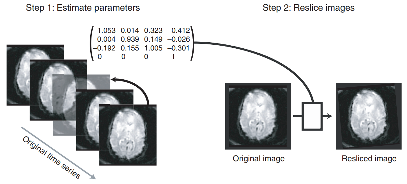
Fig. 7 Illustration of motion correction.

Hopefully it is clear that spatial motion correction is simply an image registration problem. A single fMRI volume is chosen to act as the reference image and all the other volumes are then transformed to match. As such, you can think of motion correction as a series of registration steps, where the reference stays the same and the source is changed each time to a different fMRI volume. From this perspective, there is nothing unique about the mechanics of motion correction. The main focus of most motion correction algorithms is speed, given that hundreds of volumes need to be aligned. As such, most motion correction algorithms use least-squares as the cost function. In addition, motion correction only uses a 6-parameter rigid-body transformation, which reduces the scope of the parameter space. Finally, because motions are likely to be small, the results of each previous alignment can be used as the starting point for the next alignment. As such, the optimisation algorithm should always be close to the optimal solution on each iteration, allowing it to converge quickly. As such, we can think of motion correction as simply a highly-tuned and specific version of image registration.

Motion Parameters

The registration parameters associated with each volume are one of the main outputs of motion correction. As we know, registration involves estimating a matrix \(\mathbf{T}\) that can be used to transform the source to match the target. For motion correction, there will be a \(\mathbf{T}\) matrix for each volume. Each of these \(\mathbf{T}_{t}\) matrices \((t=1,\dots,T)\) will contain the translations and rotations needed to best match volume \(t\) to the reference volume \(t^{\prime}\), where \(\mathbf{T}_{t^{\prime}} = \mathbf{I}\). The parameters of these \(\mathbf{T}_{t}\) matrices can then be used to indicate how much the subject moved during the scan. An example of these forms of plots is shown in Fig. 8.

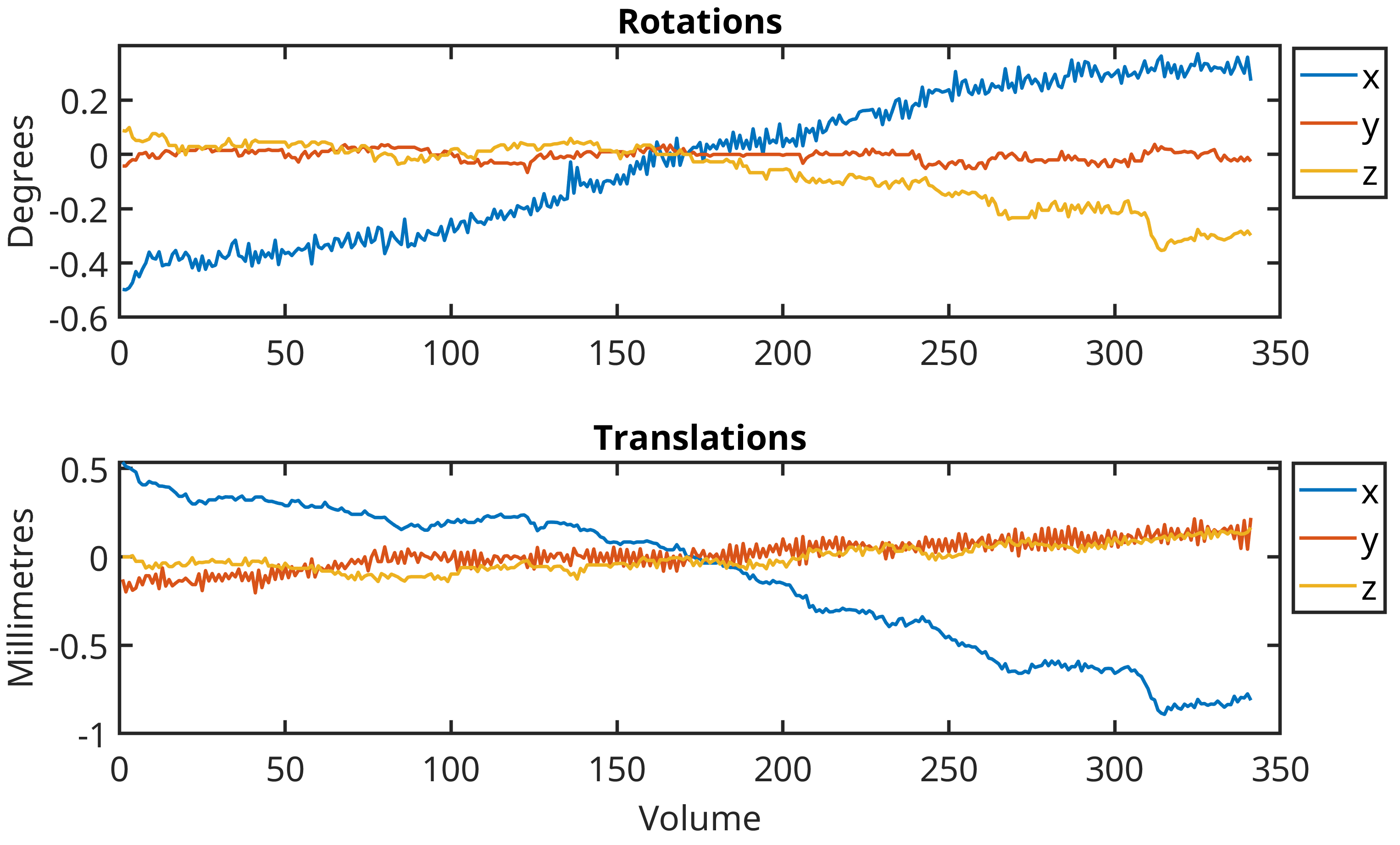
Fig. 8 Example of the plots of motion parameters produced after motion correction. In this example, the middle volume was used as the reference.

Resampling the fMRI Data

Once all the \(\mathbf{T}_{t}\) matrices have been estimated, it is typical to turn these world-space transformations into voxel-space transformations. This effectively applies the motion correction to the data by resampling each volume to match the target. Resampling at this stage is particularly important for slice-timing correction, which is our next pre-processing step. However, it is not always advisable to resample the data at this stage, as we will discussed at the end of this lesson. In terms of the interpolation itself, higher-order B-spline methods are generally preferred, as evidence suggests that linear methods can introduce greater errors (Ostuni et al., 1997). In principle, we could choose the highest-order interpolation available to us, but the gains in accuracy will likely be undone once we perform smoothing as a final pre-processing step. As such, SPM defaults to 4th-degree B-spline interpolation as a reasonable compromise.

How Much Motion is Too Much?

Considering the fact that motion is an unavoidable part of fMRI data, but is also potentially very damaging, how much motion should we allow before deciding a scan is too corrupted to use? This is an obvious question that is, unfortunately, difficult to answer. Generally, volume-to-volume motion is more damaging than steady and slow motion, meaning that motion spikes are most concerning. According to Poldrack, Mumford and Nichols (2011), a sudden shift of more than \(\frac{1}{2}\) a voxel should be cause for concern. For instance, if the voxels were 3mm isotropic then a spike of > 1.5mm in the \(x\), \(y\) or \(z\) planes would be a concern. This is similar for rotations, where we can calculate the angle for a distance of 1.5mm using the formula for the arc length of a circle

\[ \theta = d\frac{180}{\pi r} \]

where \(d\) is the distance and \(r\) is the radius. If we consider the head a circle, we can use an approximate radius of 50mm (Power et al., 2012). For 3mm isotropic voxels, this gives

\[ 1.72 = 1.5 \times \frac{180}{\pi \times 50} \]

such that any sudden rotation greater than 1.72\(^{\circ}\) would be cause for concern. However, excluding an entire scan on the basis of a single large spike would seem unwise. As such, we need to consider not only the magnitude of the motion, but also the extent of motion through the fMRI series. A couple of spikes would suggest the data is recoverable, whereas a scan that is littered with motion spikes will almost certainly be a lost cause. As an example, the plot in Fig. 9 shows a couple of concerning spikes in the \(z\)-translation trace, but this would not be enough to suggest discarding the scan. However, if similar spikes were seen across the whole series, we would be concerned about the quality of the data.

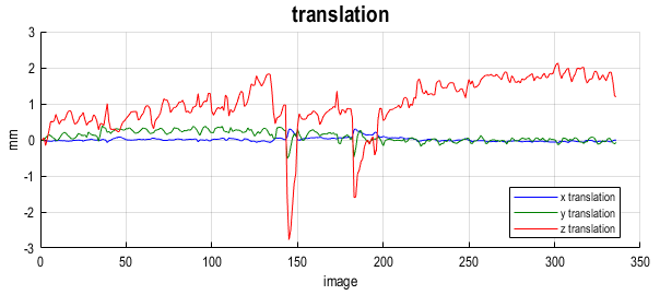
Fig. 9 Example of motion parameters containing large spikes. In this example, the spikes are not numerous enough to suggest discarding the scan.

Motion Correction in SPM

Now that we have discussed the theory of motion correction, we can examine how to perform this step using SPM.

Using the Graphical Batch System

The video below will demonstrate how to perform motion correction using the SPM graphical interface. Note that the default approach in SPM is a two-pass procedure, where the images are initially aligned to the first volume. A mean image is then created and a second pass is performed to align the volumes with the mean. The final \(\mathbf{T}_{t}\) matrices therefore represent a combination of the transformations needed for both steps. The idea is that registration can be more finely tuned using this second pass, although, realistically, it will not make a huge difference. Importantly, we need to save this mean image for use in a later pre-processing step.

Using MATLAB Code

Beyond the graphical interface, it is also possible to perform motion correction in code using the spm_realign and spm_reslice functions. For example, the code below shows how to replicate the functionality of the Realign: Estimate & Reslice module from the video.

% Launch SPM
spm('defaults','FMRI');
spm_figure('GetWin','Graphics');                  % Open graphics window for plots

% Motion correction (estimate)
func      = spm_vol('IA_preproc_func.nii');
eopts     = spm_get_defaults('realign.estimate'); % Default options struct
eopts.rtm = 1;                                    % Set to 0 for 1-pass correction

spm_realign(func,eopts);                          

% Motion correction (resample)                     
mcfunc       = spm_vol('IA_preproc_func.nii');     
ropts        = spm_get_defaults('realign.write'); % Default options struct  
ropts.interp = 4;                                 % 4th-degree B-spline
ropts.which  = [2 1];                             % [2 1] = resample all volumes (2) and create mean (1)

spm_reslice(mcfunc,ropts);

SPM12: spm_realign (v7141)                         15:21:01 - 06/11/2023
========================================================================
Printing 'Graphics' figure to:
  /home/martyn/Downloads/spm_2023Nov06.ps
Completed                               :          15:21:33 - 06/11/2023

SPM12: spm_reslice (v7141)                         15:21:33 - 06/11/2023
========================================================================
Completed                               :          15:21:51 - 06/11/2023