Step 2: Slice Timing Correction#
When it comes to acquiring a whole volume of the brain, the MRI scanner cannot do this instantaneously. Instead, the data are acquired for one slice of the image at a time, as shown in Fig. 10. These slice acquisition sequences are typically sequential or interleaved. Given that it takes a single TR to collect a complete volume, each slice within that volume will have been collected at a different time-point. For fMRI, this means that the time when the BOLD signal was sampled is going to differ depending upon the slice. Because a functional region of the brain may span multiple slices, this means that the point during that region’s response that is measured is going to depend upon which slice the region falls in. For an interleaved sequence, this could mean a difference of \(\frac{1}{2}\) TR within the same region. Such timing discrepancy can cause serious problems when it comes to the statistical modelling of fMRI data.
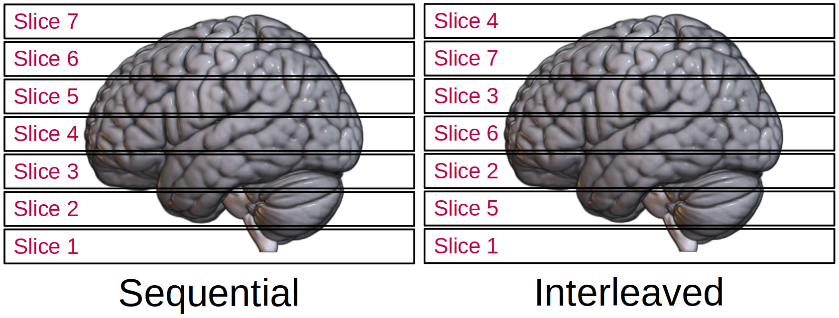
Fig. 10 Illustration of how a single volume of the brain consists of multiple slices collected at different times.#
The Slice Timing Problem#
The main issue with slice timing is that, even if the shape of the BOLD signal is the same in every slice, different points along this shape will be sampled due to the time delay from one slice to the next. This can result in the reconstructed shape of the signal being quite different from the true shape of the signal. This is illustrated in Fig. 11. On the left are 5 slices showing identical BOLD responses in blue. The samples recorded by the scanner are given by the red circles. Notice that the location of the samples differs in each slice due to the acquisition delay. On the right is the reconstructed signal inferred from the samples. For slice 1, this reconstruction is reasonably accurate. However, for slice 5, the acquisition delay has caused the peak of the signal to appear a whole TR earlier than it actually did. This is because the reconstructed signal does not take the acquisition delay into account, instead assuming that all slices were collected simultaneously. This is an issue because a standard fMRI statistical analysis will also assumes that the slices were collect simultaneously. Although this may suggest that the statistical analysis should be adjusted for each slice (as described by Worsley et al., 2002), the approach used by SPM is to instead adjust the data in each slice to meet the analysis assumptions.
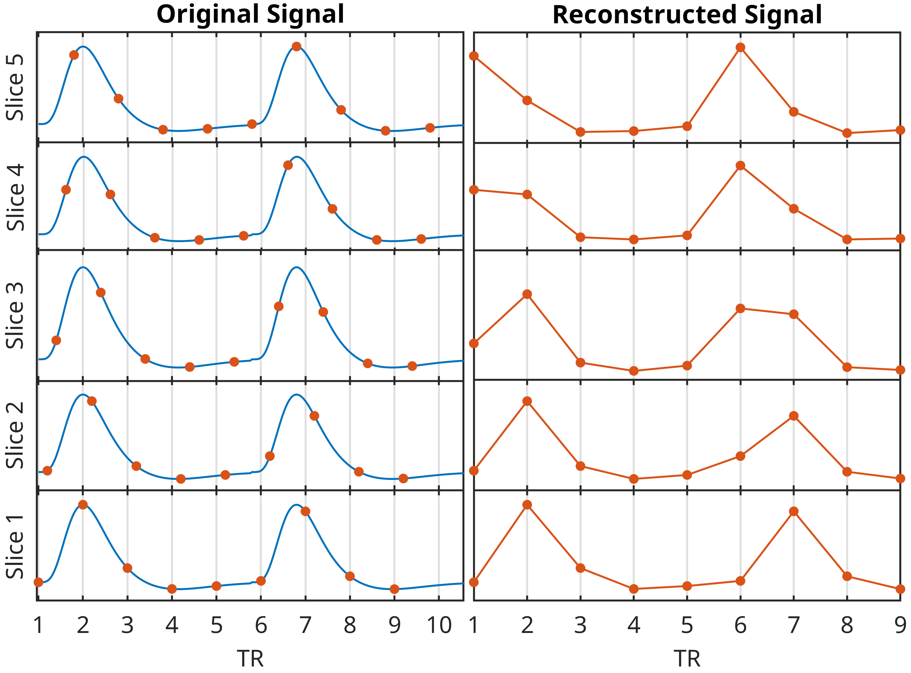
Fig. 11 Illustration of the slice-timing problem.#
Slice Timing Correction#
Slice timing correction is a method of interpolating a time series forwards or backwards in time so that it represents the signal as if it had been measured earlier or later. Doing this for each slice means we can create a dataset where all the time series data appears as if it was collected simultaneously. In order to do this correctly, we need knowledge of what order the slices were collected in and which slice to use as the reference. This reference slice represents the time that all other slices are interpolated to match. Intuitively, interpolating all the data to match the first slice seems to make sense, however, this would result in greater interpolation for later slices. As such, the middle slice is often chosen instead. This means that the whole dataset is shifted to appear as if it were collected halfway between each TR.
This process is illustrated in Fig. 12. One the left, the blue circles represent the same samples taken in Fig. 11. The curved orange line through these samples is the result of spline interpolation. The orange crosses then represent the new sampled points taken for the slice timing correction. These points match those from the middle slice (slice 3), meaning that the data should appear as if it were collected at the same time-point as the middle slice. The reconstructed signal from those new samples is then shown on the right. In theory, because the response was identical across all slices, this should look the same as slice 3 in every slice. In this example, this has only been somewhat achieved, due in part to the low sampling rate (equivalent to a TR of 5 seconds). However, the main point is that signal peaks are no longer as egregiously out-of-line as they were originally. With a greater sampling rate, these results would be even more consistent and the reconstructed signal would appear closer and closer to that of the reference slice.
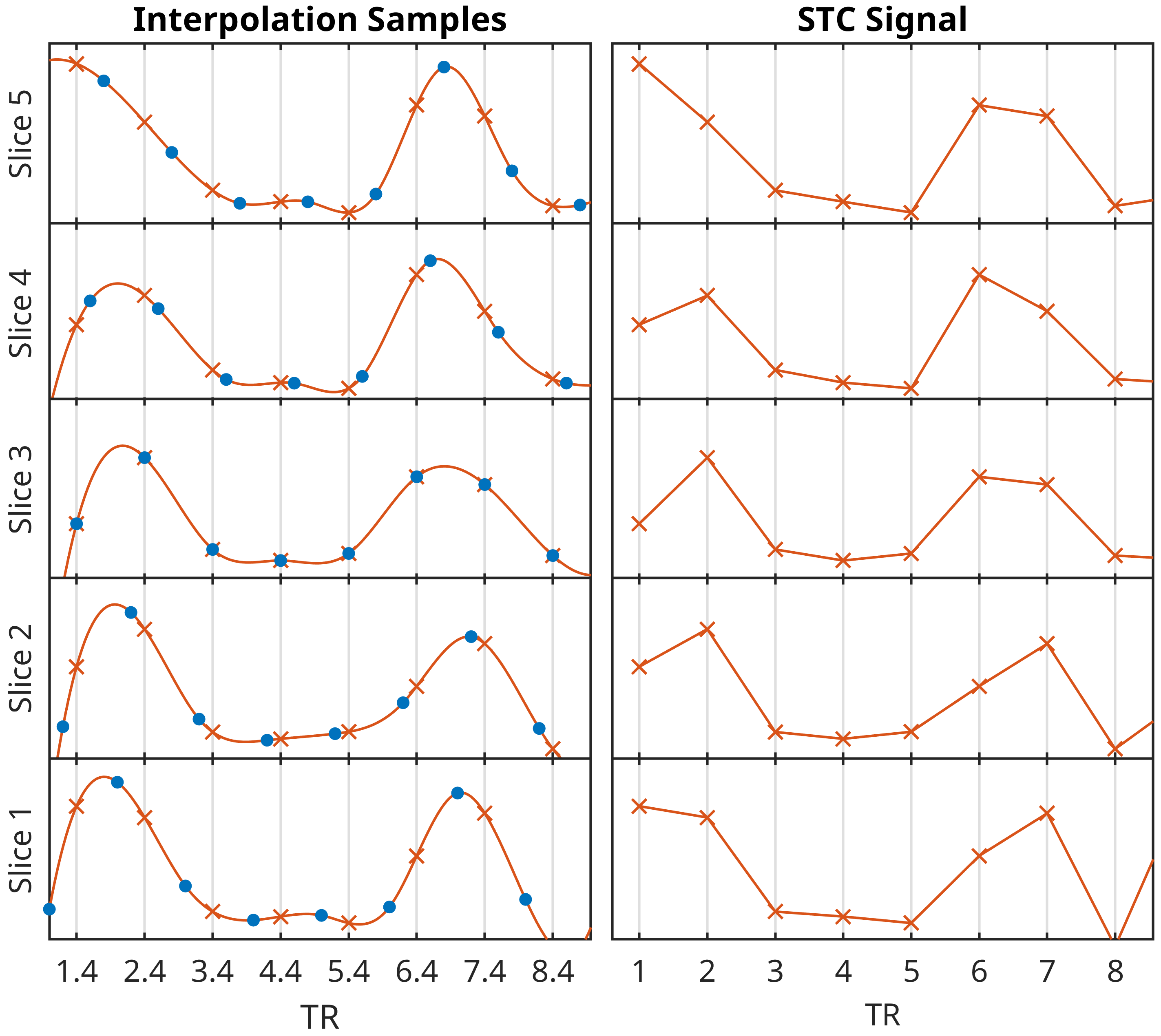
Fig. 12 Illustration of slice-timing correction.#
Warning
From a practical perspective, we need to know the acquisition sequence used to collect the data in order to perform slice timing correction. This should be known from when the scanning sequence was setup, or as part of the metadata for a particular dataset. Importantly, if this information is not available then slice timing correction cannot be used. Any attempt to guess what the sequence was will result in a correction that will destroy the time series. You have been warned.
Slice Timing Controversy#
Unlike the other preprocessing steps in this lesson, slice timing correction is contentious. One of the more general issues is that slice timing correction changes the shape of the time series at each voxel. As we will come to see, this shape is hugely important for the statistical analysis and thus any changes are likely to significantly affect the results. This means we have to be confident that slice timing correction is being applied accurately and not introducing any biases that could lead to spurious findings. Further issues with slice timing relate to the interaction between the slice acquisition offset and head motion, as well as the interpolation method employed by SPM. Of the two, the interaction with motion is particularly problematic as, depending on the amount of motion and the acquisition sequence, the ordering of motion correction and slice timing correction may need to be swapped. In terms of interpolation, SPM performs slice timing correction in the frequency domain. Though there are good reasons for doing so, this approach can lead to ringing artefacts and issues with the time series wrapping during interpolation. As such, the data must be checked carefully after slice timing correction has been applied. As a final point, the degree to which slice timing is necessary depends upon the length of the TR. Clearly a discrepancy between slices of up to 5 seconds is a bigger issue than a discrepancy of 2 seconds. Alternatives to slice timing correction exist that can be used during the statistical modelling to introduce temporal adjustments. As such, there may be cases where slice timing is avoided entirely in favour of these alternatives. We will pick up some of these points again at the end of the lesson when we start exploring how to build a preprocessing pipeline.
Slice-timing in SPM#
Now that we have discussed the theory of slice timing correction, we can examine how to perform this step using SPM. The video below will demonstrate how to perform slice timing correction on the motion-corrected functional data, using the SPM graphical interface.